
Modeling Urban Wetland Hydrology for the Restoration of a Forested Riparian Wetland Ecosystem
by Christopher Obropta1,2, Peter Kallin3, Michael Mak4,
and Beth Ravit1
1Department of Environmental Sciences, Rutgers University, New Brunswick, New Jersey 08901
2Rutgers Cooperative Extension, Rutgers University, New Brunswick, New Jersey 08901
3Belgrade Regional Conservation Alliance, Belgrade Lakes, ME 04918
4Graduate Program in Environmental Sciences, School of Environmental and Biological Sciences, Rutgers University, New Brunswick, New Jersey 08901
Abstract
To achieve our goal of a sustainable wetland system within a highly urbanized watershed, we required a model of the site's existing hydrology. This model will be used to develop a Conceptual Restoration Plan incorporating hydrology capable of sustaining the reestablished wetland system. Initial data suggests that the current system hydrology is dominated predominately by surface water flows. We have utilized the USEPA SWMM model to characterize water movement through 46 subbasins on this site. These simulated surface water flows will be used in conjunction with ground water, vegetation, and soil data to develop a Conceptual Restoration Plan for the site and to predict surface water movement through the reestablished wetlands.
Keywords: Riparian wetland ecosystem, hydrology, SWMM model, water budget, runoff, aquaclude, perched bog
Introduction
Wetlands can be highly variable ecosystems that are characterized by fluctuating water levels and the prevalence of saturated soil conditions during the growing season. Riparian wetland ecosystems are positioned downstream of headwaters and typically receive runoff from their adjacent watershed (Grayson et al. 1999; Thurston 1999). Due to urbanization that occurred during the 20th century, many wetlands in highly developed areas in the Northeast United States have been cut off from their historic water sources. The hydrology of these urban wetland systems, including the inflows from their surrounding watershed, has been radically altered (Ehrenfeld et al. 2003).
To reestablish a sustainable 20-acre urban wetland system on the 46-acre Teaneck Creek Conservancy site, it is critically important to understand the site's existing hydrology. Based on data collected from over 40 groundwater wells installed on the site, information obtained from a wetland delineation, and soil profiles taken along a transect traversing the site from east to west, we have concluded that in areas where wetlands will be reestablished, subsurface and groundwater movement is currently negligible. Surface water flows in these areas dominate the hydrology because of the presence of fill materials, including a clay berm located adjacent to Teaneck Creek and a clay layer underlying most of the site at depths of 1 to 4 feet. Due to these historical disturbances, the wetland system currently appears to be functioning as a perched bog rather than a riparian corridor wetland. Therefore, we have prioritized characterization of surface water flow and development of a model to simulate these flows as the first step in determining pre-restoration baseline hydrology.
A comprehensive water budget is necessary to characterize the hydrology of an urban wetland system, but it is difficult to estimate the various components of urban hydrology or to create hydrologic simulations over extended time periods (Drexier et al. 1999). Although some water budgets have attempted to describe wetland hydrology (Konyha et al. 1995; Reinelt and Horner 1995; Hawk et al. 1999; Arnold et al. 2001; Kirk et al. 2004; Zhang and Mitsch 2005), models capable of describing urban wetland water flows are extremely few (Drexier et al. 1999; Raisin et al. 1999). We are aware of only one peer-reviewed study (Owen 1995) that attempted to develop a comprehensive urban water budget. This data gap is especially critical since current wetland modeling is derived from traditional pond design engineering (Konyha et al. 1995), which is a serious limitation when modeling wetland water fluctuations that are typically more subtle than water movement captured by pond models.
Lack of reliable data creates a challenge in determining how an urban wetland interacts with the adjacent watershed. Development of a hydrologic model that can accurately describe a given urban wetland is a necessary first step in the successful reestablishment of sustainable wetlands on a restoration site. The goal of this study was to characterize surface water movement as it currently exists in the urban wetlands of Teaneck Creek.
Modeling the Urban Teaneck Creek Surface Waters
Surface hydrology, in conjunction with groundwater hydrology and soil characteristics, controls the hydrology budget of a wetland. In highly urbanized locations such as the Conservancy site, the input of stormwater runoff into local wetlands is a potentially critical component of the water budget. High amounts of impervious cover (roofs, road surfaces) in urban areas increase stormwater runoff velocities and volumes. These increased velocities produce water budgets that differ from those of wetlands in non-urban settings (Göbel et al. 2004). Urban surface water inflows to the Conservancy site occur via both stream overbank flow and from six storm drains that discharge directly into the wetland system. Precipitation is most likely the dominant factor in a hydrologic simulation of the Conservancy's wetlands.
The basic hydrologic parameters of wetland water budgets include surface water influxes, precipitation, groundwater influxes, storage of water, percolation, and evapotranspiration (Owen 1995; Hawk et al. 1999; Reinelt and Horner 1995). There are three approaches used to model wetland hydrology: single event models, stochastic models, and comprehensive water budgets (Koob et al. 1999). The mass balance approach provides a framework for developing a water budget, which seeks to incorporate the parameters that control a wetland's hydrology. Further generalizations or additional parameters, such as a proposed restoration design of the system's hydrology may also be included in a model (Owen 1995; Reinelt and Horner 1995; WDWBM 1997; Yu and Schwartz 1998; Drexier et al. 1999; Raisin et al. 1999; Kincanon and McAnally 2004; Göbel et al. 2004; Mo et al. 2005; Xiong and Melching 2005; Zhang and Mitsch 2005).
Because urban hydrology may be subject to more highly fluctuating environmental conditions than a non-urbanized system, there may be an advantage in applying a stochastic model to urban wetlands, since this model type allows the incorporation of uncertainty into the model results. This approach contrasts with deterministic models, which produce identical results when provided with constant input parameters. Another alternative is to use a deterministic model with variable inputs to examine a range of conditions (e.g., dry conditions, wet conditions, average conditions).
Teaneck Creek Surface Water Hydrology
If an urban wetland system is characterized by minimal or nonexistent groundwater interactions, then the urban wetland may require a non-traditional modeling approach. In urban systems where the groundwater component is minimal, the most effective modeling approach to simulate hydrologic conditions may be the application of a nonlinear reservoir method, such as the United States Environmental Protection Agency Storm Water Management Model (SWMM). SWMM is a comprehensive deterministic model for urban stormwater runoff, capable of considering both water quality and quantity during a single event or on a continuous time frame (Huber and Dickinson 1988; Tsihrintzis and Hamid 1998; Bhaduri et al. 2001; Burian et al. 2001; Choi and Ball 2002; Lin et al. 2006; Smith et al. 2005; Xiong and Melching 2005). SWMM is designed to simulate real-time storm events based on spatial and temporal rainfall, evaporation, topography, impervious cover, percolation, depression storage values for impervious and pervious regions, storm drainage attributes such as slope and geometry, Manning's n, and infiltration rates (Burian et al. 2001; Bhaduri et al. 2001; Choi and Ball 2002). Based on these parameters, SWMM will model infiltration and storage and divert the remaining runoff as sheet flow (Burian et al. 2001). SWMM includes four simulation blocks to model urban stormwater runoff: Runoff; Transport; Extran; and Storage/Treatment.
When integrated with a GIS platform, SWMM is capable of developing simulations for defined subwatersheds existing within the boundaries of a given system. The watershed boundary is divided into smaller subdivisions based on land use, soil characteristics, impervious attributes, and topography (Smith et al. 2005), and this allows SWMM to generate runoff hydrographs based on daily rainfall data for each delineated subwatershed (Smith et al. 2005). An inflow of precipitation data will produce outflows of infiltration, evaporation, and surface runoff. Surface runoff will occur when each subbasin or reservoir reaches maximum storage. The depth of water for each subcatchment will be calculated continuously over the desired time step, through continuous calculations of the water balance. For each subwatershed, SWMM can simulate an individual rainfall event or a continuous simulation in time steps of minutes to years based on the system being modeled.
The SWMM model exhibits the highest potential to accurately simulate hydrological processes occurring within an urban wetland, and would thus be able to provide a solid framework for developing an accurate water budget for an urban wetland system. Through SWMM, the characteristics that define urban wetland systems with limited groundwater influences may be simulated on a continuous basis, providing a comprehensive description of the interaction of urban wetlands with the surrounding watershed. For these reasons, we chose SWMM to model the Teaneck Creek water flows. We chose to simulate the response of the Conservancy wetlands over a five-year period that included wet, dry, and average meteorological conditions (Table 1).
Materials and Methods
Click image to enlarge
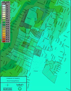
Figure 1: Sewershed System based on the Township of Teaneck Digital Elevation Model (DEM) — 10 meter.
The wetlands on the 46-acre Teaneck Creek Conservancy site were delineated based upon vegetation, soils, and hydrology (Ravit et al. this volume). Soil characteristics of these wetlands have been highly modified by anthropogenic activity during major roadway construction in the 1950s and by current urban conditions (Arnold this volume), and these soil attributes are incorporated into the infiltration calculation in the SWMM model. Sewer system record survey maps of the Township of Teaneck (1972), 2002 NJDEP Orthoimagery, and 10-meter and 2-foot Digital Elevation Models (DEMs) were obtained to delineate the extent of the sewersheds draining into the wetland using ArcGIS 9.0. We analyzed the 10-meter DEMs, in conjunction with the invert elevations of the storm sewer lines in the township, to define the catchments and to provide the basis for assigning individual drainage areas to each catch basin. We delineated a total of 46 sub-sewersheds within the sewershed draining into the Conservancy wetland (Figure 1) and the size and slope characteristics of each were determined in ArcGIS.
Click image to enlarge
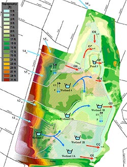
Figure 2: Surface water routing through Teaneck Creek Conservancy wetlands. S = inflows to the Conservancy wetlands; O = outflows from the Conservancy wetlands.
The 46 sub-sewersheds (subcatchments) with their corresponding attributes and dimensions were constructed in EPA SWMM 5.0. The attributes of the subcatchments required to run a storm simulation consist of: area; width; slope percentage; percentage of imperviousness; infiltration method; and the outlet junction. The NRCS TR-55 SCS curve number infiltration method was used, based on the 1/8-acre or less (65% imperviousness) average residential lot size and the particular hydrologic soil group existing in each sub-sewershed (SCS 1986). The hydrologic soil group of each sub-sewershed was provided by the NRCS SSURGO soils data layer imported into ArcGIS 9.0. Once the entire sewershed was defined in SWMM, the six outfalls of the sewer lines and sub-sewersheds were modeled to complete the storm sewer portion of the system. The wetland subcatchments were then created using 2-meter DEMs within the boundary of the Conservancy. The attributes for the subcatchments were measured through ArcGIS 9.0 and imported into SWMM. Six subcatchments were delineated within the site, some of which flowed in different directions depending on the water elevations within the basins. This was simulated in SWMM using weirs and diversion structures, and each wetland basin was modeled as a pond with storage defined by the topography.
Click image to enlarge
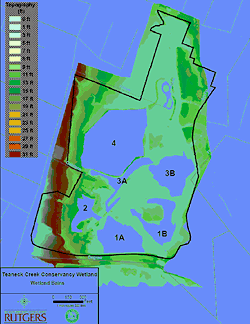
Figure 3: Teaneck Creek Conservancy wetland areas.
There are six stormwater inflows to the wetland and eight locations where water discharges to the Teaneck Creek and its tributaries. Figure 2 is a graphical representation of the predicted surface water routing through the wetland and Figure 3 shows the geographical location of the various wetland basins. Routing of water from the sewer system through the wetland and into Teaneck Creek was predicted using the 2-foot GIS contours for the wetland. This routing was field-verified by on-site visits during two rainfall events. Complete details of the SWMM model can be found in Mak (2007).
Model Field-Calibration
Two rainfall events were recorded at a representative location of the modeled system. A pressure transducer and a rain gauge were installed at Stormwater Canyon (S-1 in Figure 2), which receives runoff representative of the other sub-sewersheds within the drainage system and is the primary source of water to the largest wetland area that will be reestablished. The rainfall events were input into SWMM to calibrate the model through a comparison of the predicted flow versus the actual flow measured during these two storm events. The pressure transducer recorded water depth throughout the storm at 4-minute intervals, requiring a rating curve to calculate the actual flow through the canyon. Previously recorded Stormwater Canyon flow measurements were used to develop the rating curve for the two storm events. The recorded rainfall data were input into SWMM with the corresponding dates and time steps of the storm events. The output data from each simulation were then imported into Microsoft Excel for model validation. For these storm events, two subsets of simulations were run for the model calibration. The parameters adjusted during the calibration of the model were the curve numbers representing the infiltration routing processes, the percentage of impervious area with no depression storage, and percentage impervious cover values for each subbasin in the sub-sewershed under review. Plots of observed versus measured flow for each calibration simulation were then analyzed for the validation of the model.
Validation
Click image to enlarge
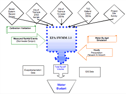
Figure 4: Logic flow for model development and water budget calculations.
To validate the model, we used a numerical integration method (trapezoidal rule) to analyze the measured versus predicted values. We calculated the total runoff volume for each simulation using the trapezoidal rule and compared this to the measured flows. At the calibration point, the measured versus predicted values for total runoff volume differed by only 2.06% (Mak 2007).
Water Budget Calculations
Once the model was calibrated and validated, we used it to generate annual rainfall simulations to develop a water budget. To simulate an annual rainfall event, 15-minute and hourly precipitation data in DSI-3260 and DS-3240 format, respectively, were imported into SWMM. Due to completeness of the data set and relative proximity to the project site, the precipitation records from Newark Airport (Table 1) were used for these annual simulations. Figure 4 shows the overall logic flow of how the model was developed and used to calculate annual water budgets.
The SWMM model was used to predict the volume of water draining into and out of the TCC wetland from the surrounding sewershed. Using this information, we created a monthly water budget for the entire wetland for the years of 2000 through 2005. The calculation of the water budget was done in Microsoft Excel using runoff data imported from EPA SWMM 5.0, the New Jersey State Climatologist (http://climate.rutgers.edu/stateclim_v1/monthlydata/index.html), and the National Climatic Data Center (NOAA) (www.ncdc.noaa.gov). The calculation of the water budget follows a mass balance approach provided by Mitsch and Gosselink (2000) and Owen (1995). The general mass balance exists as (change in storage = input – output). The mass balance applied to the wetland is derived from the expression:
Equation 1: Water Budget Equation
ΔS = P + Si + Gi – AET – I – So – Go ± T
Where:
ΔS = change in storage volume
P = precipitation
Si = surface water inflow
Gi = ground water inflow
AET = actual evapotranspiration
I = infiltration
So = surface water outflow
Go = ground water outflow
T = tidal flow
For each annual simulation, surface water inflows (Si) and outflows (So) in cubic feet per second (CFS) were imported from EPA SWMM 5.0 and converted into units of acre-feet for the water budget calculations. Hourly precipitation values (DS-3240 format) from Newark International Airport (Station #286026) were obtained from the National Climatic Data Center (NOAA) (www.ncdc.noaa.gov) for the years 2000 through 2005. The Newark station is located approximately 16 miles from the Conservancy wetlands and contains the most complete hourly rainfall data sets of any station in the vicinity. The precipitation (P) inputs for the wetland itself were calculated by summing the hourly data (in inches) and converting to acre-feet.
Potential evapotranspiration (PET) was calculated on a monthly basis using the Thornthwaite equation (Mitsch and Gosselink 2000):
Equation 2: Potential Evapotranspiration (PET)
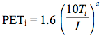
PETi = PET for month I (mm/mo)
Ti = mean monthly temperature (°C)
I = local heat index, 
A = (0.675 × I3 – 77.1 × I2 + 17,920 × I + 492,390) × 10-6
We chose the Thornthwaite method because of its simplicity and reasonable accuracy (Mitsch and Gosselink 2000). Only air temperature is required to derive values for PET occurring within the wetland. Air temperature data were retrieved from a continuous weather monitoring station located in Lyndhurst, New Jersey, approximately 10 miles from the Conservancy. These data were provided by the Meadowlands Environmental Research Institute (MERI). Data were retrieved from this station because of its close proximity to the project area and the availability of the data. Actual evapotranspiration (AET) values were derived by applying a correction factor to the calculated PET.
Click image to enlarge

Figure 5: Cumulative monthly water budget for the period 2000–2005.
For the purposes of this simulation, we assumed groundwater inflows (Gi) to be negligible and did not include them in water budget calculations. Although there is some evidence of groundwater movement in portions of the wetland, a highly impermeable clay layer exists underneath much of the system, minimizing the influences of ground water. The existence of a dense clay layer under most of the wetland acts as an aquaclude and causes the system to act essentially as a perched bog, with some infiltration into surficial sediments above the clay layer and very slow movement toward the creek. We have observed a few seeps along the creek bank in several areas that flow for a few days after large rainfalls, which support this assessment. These infiltration losses (I) were calculated by SWMM based on the soil characteristics in the wetland basins and converted from inches to acre-feet. We calculated the total infiltration loss for the entire system by summing the values for the individual wetland basins for each month during the 6-year simulation period.
All of the model inputs and collected data were imported into Excel to compute the monthly budgets for the years 2000 through 2005 to simulate the current conditions of the existing wetland. We combined monthly precipitation totals and simulated runoff totals to represent the total inflow into the system, and we combined actual evapotranspiration, infiltration loss into the wetland, and simulated outflow totals to represent the total outflow from the system.
Results
Click image to enlarge
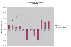
Figure 6: Average monthly Teaneck Creek Conservancy water budget for the period 2000–2005.
The change in storage of the system each month was calculated by subtracting the total outputs from the total inputs of the system. This represents the amount of water stored in or removed from the wetland system each month. To calculate the cumulative storage for the wetland system, we added the change in storage for each month to the previous month's cumulative storage, resulting in the cumulative storage plot shown in Figure 5. Table 1 summarizes the monthly and annual precipitation values for the six-year period of analysis. Years 2000 (44.45 inches) and 2005 (47.78 inches) were slightly below the six-year mean precipitation (51.06 inches); the amount of water in the wetland at the end of those years was roughly the same as at the beginning. Year 2001 (37.47 inches) was the driest year analyzed; the wetland ended the year with a deficit of about 70 acre-feet compared to the beginning of the year. This deficit did not fully recover until the end of 2003 (54.77 inches), which was the wettest year in the period analyzed.
We averaged the monthly change in storage values (all Januaries, all Februaries, etc.) over the six years to generate average monthly storage changes. These are shown in Figure 6, along with the cumulative plot of the average values. During "average" precipitation years, the wetland gains water in the spring and fall and loses water in the summer. The detailed data used for calculations of the water budget are included in Mak (2007).
Discussion
A methodology has been developed for analyzing the water budget of the Teaneck Creek urban wetlands, based on a surface water–dominated system. While the results presented here are for the entire TCC wetland complex, the SWMM model can be used to analyze water budgets for each of the individual wetland basins shown in Figure 3. The model can be used to analyze each wetland basin, separately or in combination, and to evaluate the effects of various restoration options, such as grading changes or installing water-control structures. Also, the model can be used in combination with water quality data to analyze nutrient loadings to various areas within the wetland.